So you want to plot a global geoTIFF in web mercator...

Nov 10, 2022 · 7 min read

Need to go from epsg:4326 to web mercator and you’re a bit of a GIS n00b like me? Read on!

This week I found myself in the following situation: I had a geoTIFF of a NASA data product and I needed to get that geoTIFF into a web-ready format. The main trickiness here was that the geoTIFF was a global image in a standard epsg:4326 cooredinate reference systems and most web-app mapping tools work in a web mercator projection (epsg:3857). And while I remembered that web mercator isn’t great near the poles, I didn’t realize just how bad it was…

In this post, I’ll walk through the problem of re-projection, first showing you what not to do (and why it’s bad) before showing you a nice way to re-project a geoTIFF and save off a bitmap image.

For other mapping-related work, I’ve used the rasterio python package and found it generally a great tool, and so that’s what I’ll be using here.

Packages

This the code here requires the following:

rasterio
matplotlib
numpy
pyproj
PIL

all of which are available via pip or conda.

Data

For this notebook, we’ll use some sample data from NaturalEarthData. Importantly, this is a global raster, covering longitude from -180 to 180 degrees and latitudes from -90 to 90 degrees. The exact dataset can be downloaded from:

https://www.naturalearthdata.com/downloads/10m-raster-data/10m-gray-earth/

The following uses the large, “Shaded Relief, Hypsography, Ocean Bottom, and Drainages” version. Download and unzip the folder and update the filepath in this notebook if necessary.

Initial Data Inspection

Let’s start by loading the .tif file and plotting what we have:

import rasterio as rio
import matplotlib.pyplot as plt

fpath = "GRAY_HR_SR_OB_DR/GRAY_HR_SR_OB_DR.tif"

src = rio.open(fpath)
im = src.read(1)

plt.imshow(im, cmap="plasma")

png

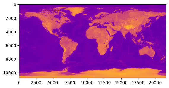
We can check the coordinate reference system to see that we are indeed in epsg:4326:

src.crs

CRS.from_epsg(4326)

and we can check the bounds with

src.bounds

BoundingBox(left=-180.0, bottom=-90.000000000036, right=180.00000000007202, top=90.00000000000001)

and some more metadata:

src.profile

{'driver': 'GTiff', 'dtype': 'uint8', 'nodata': None, 'width': 21600, 'height': 10800, 'count': 1, 'crs': CRS.from_epsg(4326), 'transform': Affine(0.01666666666667, 0.0, -180.0,
       0.0, -0.01666666666667, 90.00000000000001), 'blockysize': 1, 'tiled': False, 'interleave': 'band'}

So we see that there’s a single band (since this a greyscale image) and the bounds do indeed grom from +/-180 longitude and +/-90 latitude.

Projecting to web mercator EPSG:3857

Ok, so now maybe we want to use this nice image as a base layer in some mapping web-app like MapBox, Leaflet, or any number of other web-based mapping service. Many of these services do provide some of their own projection/transformation methods, but often it’s easier to just pre-compute the projection so that you have an image that’s already in the expected web mercator projection.

Projecting (or re-projecting) with rasterio is very straightforward. rasterio’s documention on Reproduction even covers this exact case where we what to go from 4326 to 3857! Easy peasy, right?

So let’s just naively follow the rasterio example. First, let’s set our destination coordinate reference:

dst_epsg = 3857
dst_crs = rio.crs.CRS.from_epsg(dst_epsg)

and now we calculate the transform needed to go between our source and destination crs. THe following function also computes the resulting width and height of the image:

from rasterio.warp import calculate_default_transform
transform, width, height = calculate_default_transform(
    src.crs, dst_crs, src.width, src.height, *src.bounds)

ok, let’s check the size of our new image…

(src.width, src.height)

(21600, 10800)

hmm, the width is about twice the height. well, I dunno, maybe that’s right. Let’s keep going!

Next, first iniitalize an empty array of our expected height and width, and then we reproject into that array (rather than writing a new file, like in the rasterio example):

from rasterio.warp import reproject, Resampling
import numpy as np

dst_array = np.empty((height, width))

_  = reproject(
    source=src.read(1),
    destination=dst_array,
    src_transform=src.transform,
    src_crs=src.crs,
    dst_transform=transform,
    dst_crs=dst_crs,
    resampling=Resampling.nearest)

great! now we’re ready to plot!

plt.imshow(dst_array, cmap="plasma")

png

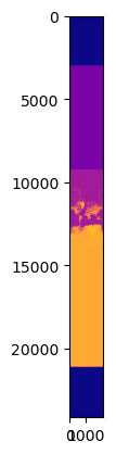
well. hmm. that’s… something? At least the continents are there?

web mercator limits

Well, all you GIS non-n00bs are probably laughing by now, because you know. But it took me a while to realize what was happening.

The issue actually comes straight from the definition of web mercator! You can check this NGA PDF documentation for a real deep dive, but in slightly simplified form (with no offsets), the x-axis (or the “easting” direction) is calculated with:

E = a * lon_radians

where a is the semi-major axis of the reference ellipse used (the earth’s mean radius!) and lon_radians is the longitude in radians.

For the y-axis, the “northing” direction, we have:

N = a * ln(tan(pi/4 + lat_radians/2))

where lat_radians is the latitude in radians.

And that tangent there is where we’re running into trouble with our reprojection, because as latitude approahces +/-90, we’ll be hitting that discontinuity, which is what’s causing our map to stretch out like crazy. Let’s use pyproj to actually show the northing direction as you approach the poles:

from pyproj import Transformer

transformer = Transformer.from_crs("epsg:4326", "epsg:3857")

lon = np.full((1000,),-180)
lat = np.linspace(80,89.99999, 1000)
x, y = transformer.transform(lat, lon)
plt.plot(lat, y)
plt.xlabel("latitude")
plt.ylabel("northing axis")

png

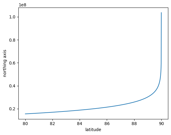
yikes!

So that’s why, when you look up info on web-mercator, it gives the map bounds as +/-85 degrees latitude or so (wikipedia says google uses +/-85.051129 degrees).

If we just plot from +/-85, we see that the variation is nicely defined:

lon = np.full((1000,),-180)
lat = np.linspace(-85,85, 1000)
x, y = transformer.transform(lat, lon)
plt.plot(lat, y)
plt.xlabel("latitude")
plt.ylabel("northing axis")

png

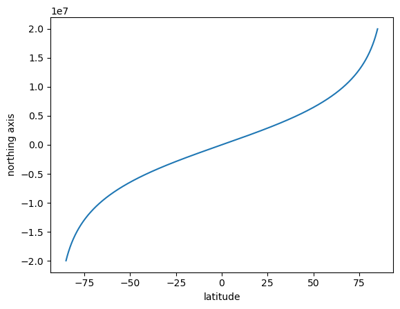
There’s still some nonlinearity that causes the poles to stretch but as most web-mapping applications are concerned more with human habitation, the distortion at the poles is not such a big deal.

re-projecting the rigth way

OK! So back to the problem at hand!

The thing to realize is that rasterio does not enforce the +/-85 degree range and we need to account for that! Note that I’m not saying rasterio should account for it, there’s a good argument to requiring users to clip their own data in ways that are appropriate for their use case. But it does require you to remember the limits here!

The solution is to of course clip our geoTIFF to avoid the problematic poles. We can do this by building a rasterio Window to use in the transformation.

First, let’s initialize a window using a BoundingBox:

clip_box = rio.coords.BoundingBox(-180., -85., 180., 85.)
clip_window = src.window(*clip_box)

and let’s round that window (in case we’ve selected lat/lon ranges that fall between pixels) and then pull out the height and width of our window:

clip_window = clip_window.round_lengths()
window_height = int(clip_window.height)
window_width = int(clip_window.width)

(window_height, window_width)

(10200, 21600)

the other key is that rather than using the src.transform in our call to reproject, we need to build a window_transform that takes into account the clipping that we want:

window_tform = src.window_transform(clip_window)

and now we’re ready to calculate the source to destination transformation (where we are suppling the clipping window properties):

transform, width, height = calculate_default_transform(
    src.crs, dst_crs, window_width, window_height, *clip_box)

(width, height)

(16919, 16863)

and we get something much closer to square (as you should for a web-mercator global projection).

So now let’s finish up our transform. Not that we are suppling the window transform as the src_transform here:

dst_array = np.empty((height, width))

_  = reproject(
    source=src.read(1),
    destination=dst_array,
    src_transform=window_tform, # important! no longer src.transform,
    src_crs=src.crs,
    dst_transform=transform,
    dst_crs=dst_crs,
    resampling=Resampling.nearest)

plt.imshow(dst_array, cmap="plasma")

<matplotlib.image.AxesImage at 0x7f305e6ba020>

png

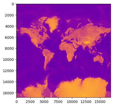
that’s much better, isn’t it??

Exporting as a PNG

So now, we have our data projected into web-mercator and stored in that dst_array, from where you could do any number of things. One likely use case is that you want to save off a bitmap of this to use as a base layer in a web app… So let’s do that!

Let’s start by applying a colormap to our re-projected data array. First we need to scale between 0,1 then apply a matplobli colormap and cast the result as integers between 0 and 255:

from matplotlib import cm

scaled_dst = (dst_array - dst_array.min())/(dst_array.max() - dst_array.min())
scaled_dst = cm.plasma(scaled_dst)
scaled_dst = np.uint8(scaled_dst*255)

And now we can initalize our PIL.Image. We’ll also resize at fixed aspect ratio (cause I don’t need a 100MB+ png in my life), then save (and display again):

from PIL import Image

new_width = 500
img = Image.fromarray(scaled_dst)

height_over_width = float(img.size[1]) / img.size[0]
new_height = int(height_over_width * new_width)

img = img.resize((new_width, new_height), Image.Resampling.LANCZOS)
img.save('rescaled.png')
img

png

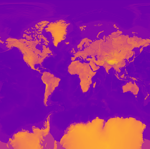
And a small image like that is easy to encode and send over the web as needed! And it’s already in web mercator, ready for use as a global base layer.

summary

So remember folks, clip before projecting!

Happy mapping!