Specifying unrelaxed moduli in the VBRc (version 1.1+)

Jan 4, 2024 · 9 min read

The most recent feature release of the VBRc (version 1.1) included some changes that simplify the specification of the unrelaxed moduli used within the VBRc. These changes allow you to directly specify the unrelaxed shear and bulk moduli at the temperature and pressure of interest and have those values automatically used in rest of the workflow, including subsequent elastic methods (like the poroelastic calculation) and in the calculation of relaxed moduli. This post demonstrates how to use this new feature by using the MATLAB code from the Abers and Hacker 2016 MATLAB toolbox to calculate the unrelaxed shear and bulk moduli (and density!) that get passed into the VBRc.

Background: anharmonic dependence and the VBRc

Since the VBRc was designed primarily for calculating anelastic effects (which don’t kick in until relatively high temperatures), the default anharmonic calculation in the VBRc uses a linear scaling of the elastic moduli. Comparing predictions from the VBRc to observed seismic properties, however, can require calculating properties over large temperature and pressure ranges and the linear anharmonic scaling can introduce errors over these large ranges. One consequence, for example, is that if you calculate seismic velocities for a 1D temperature profile from the surface of the earth down into the asthenosphere, the predicted velocities in the shallow lithosphere can be hard to match to observations. While the linear behavior is accurate for high temperatures, at lower temperatures the dependence is not linear and a more accurate calculation is needed (for a nice review of why, including a review on the atomic origins of anharmonicity, check out section 3 of Isotta et al. (2023)). Additionally, while the VBRc’s anelastic methods do not generally apply to compositions other than olivine at present, when comparing VBRc output to observations it can be helpful to include compositional variations to, for example, add a crust to the shallow lithosphere where intrinsic anelastic effects are negligible.

To overcome these limitations, Josh Russel recently worked on a pull request to allow the VBRc to accept inputs for the shear and bulk moduli more easily. The implementation adds new input fields to the VBR structure so that you can set the shear and bulk moduli at your thermodynamic state in any way you choose. While we could have written a new method to more accurately account for anharmonic dependence at lower temperatures, there are already a plethora of tools out there that do that calculation! In Josh’s case, his workflow involves using Perple_X to pre-compute pressure-temperature look up tables that are then sampled in his MATLAB VBRc scripts, but you could instead leverage some other community code or write your own function to use. In the example here, I’ll walk through a workflow that is confined completely to MATLAB: using the Abers and Hacker 2016 database and accompanying toolbox to calculate the unrelaxed moduli and density at a range of pressures and temperatures and then feeding those results into the VBRc as inputs.

Abers and Hacker 2016

Abers and Hacker (2016) is an update to the earlier database and excel workbook for calculating seismic properties from Hacker and Abers (2004) that includes a MATLAB implementation of the same calculation. For details of the calculation, see Hacker and Abers (2004), but in brief, the calculation relies on a more complete description of anharmonic dependence that scales with the Grüneisen parameter. The Grüneisen parameter relates anharmonic variations in interatomic potential to elastic moduli (again, see Isotta et al. (2023) section 3 for a nice review with helpful figures) and is valid for wider temperature ranges than the linear scaling used by default in the VBRc. And because Abers and Hacker released a MATLAB version of this calculation, we can very simply plug build a MATLAB-only forward calculation that uses Abers and Hacker for the anharmonic calculation and the VBRc for the anelastic portion of the calculation.

The demo!

So to recap, here’s an overview of what we’re aiming to do:

specify temperatures (T) and pressures (P) of interest
use Abers and Hacker to calculate bulk modulus, shear modulus and density at the T and P of interest
pass those moduli, density and same T,P into the VBRC (along with additional independent state variables needed for the anelastic calculation).

I’ve implemented the above steps in full in this github repository. You can check out the repository README for a full description of how to setup and run the example, but I’ll walk through the main features here. And note that all of this code runs in GNU Octave as well as MATLAB, so you don’t need a MATLAB license.

The main driving script in the repository is vbrc_with_abers_hacker_anharmonic.m and a second .m file includes a function, calculate_unrelaxed_moduli_density.m, that is based off of the Abers and Hacker 2016 script, ABERSHACKER16/rockvelcalculate.m.

Initialization in `vbrc_with_abers_hacker_anharmonic.m`

The main script begins with an Initialization section that sets up some paths and sets all the variables for both calculations.

First, we need to add the directories of both the VBRc and the Aber and Hackers 2016 code (available in the supplemental materials of their paper) to the MATLAB path. I tend to store my VBRc directory in an environment variable, but you can change these lines to wherever the VBRc resides on your system (as an aside, if you don’t want to set environment variables or remember where the VBRc lives, you can always add a MATLAB startup.m file that adds the path automatically when starting MATLAB, see here):

# add relevant paths : change these as needed
addpath(getenv('vbrdir'))  # the VBRC installation directory
addpath("ABERSHACKER16")  # The Aber & Hackers 2016 directory
vbr_init();

We’re going to calculate properties for a 2D temperature-pressure grid, so next we set some 1D arrays to cover the ranges we want:

% Set conditions for anharmonic calculation
T_K_1d = linspace(1000, 1773, 10); % temperature range
P_GPa_1d = linspace(1, 4, 15); % pressure range

To use the Abers and Hacker code, we also need to specify compositional parameters. Later on in the code, I hard code in parameters that set the minerals of interest to forsterite (Fo) and fayalite (Fa), but to demonstrate how to work in some compositional changes I include an initialization variable that sets the volume fraction of Fo and Fa:

fo_fa_vol_frac_modes=[90 10]; % nominal volume fraction of Fo and Fa

These are “nominal” volume fractions, because they will be corrected to account for molar volumes later on.

Next, we’ll set all of our variables and methods needed for the VBRc calculation:

% frequency range for VBRc anelastic calculation
frequency_Hz = logspace(-5, -1, 50);

% additional state variables required for VBRc anelastic calculation, treated as
% constants in this example
constants.phi = 0.0;
constants.sig_MPa = 0.1;
constants.dg_um = 0.01 * 1e6;

% method selection for the VBRc calculation for anelastic properties
VBR.in.elastic.methods_list={'anharmonic';};
VBR.in.anelastic.methods_list={'eburgers_psp';'andrade_psp';};

A couple notes on the final 2 lines. First, when specifying the elastic moduli directly, we still need to include the anharmonic method in VBR.in.elastic.methods_list – that method now includes a check for if the bulk and shear modulus have been set. Second, in this script, we’ll use 2 anelastic methods: the Extended Burgers and Andrade pseudo-period scalings from Jackson and Faul (2010).

Calculating unrelaxed moduli

We’re now ready for the first calculation. In the main driver, this gets offloaded to a second function:

% Step 1: calculate anharmonic moduli and density with Abers & Hacker 2016
[T_K, P_GPa, G, K, rho] = calculate_unrelaxed_moduli_density(T_K_1d, P_GPa_1d, fo_fa_vol_frac_modes);

That calculate_unrelaxed_moduli_density function is based on the Abers and Hacker 2016 ABERSHACKER16/rockvelcalculate.m script, which I expanded to loop over all our temperature and pressure conditions. For each temperature and pressure, it includes 2 calls to ah16_rockvel: the result of the first includes the densities for each mineral mode at the temperature and pressure of interest, which is used to correct the volume fractions. The corrected volume fractions are then used to calculate the final effective moduli.

Anelastic calculation with the VBRc

Once we have the moduli and density, we have to set up the VBRc calculation using these values. First, we copy references to the density, pressure and temperature arrays to the expected fields in the state variable input structure, VBR.in.SV:

% fist set state variables: copy over Abers and Hacker inputs and outputs.
% state variable inputs go in VBR.in.SV:
VBR.in.SV.rho = rho;
VBR.in.SV.P_GPa = P_GPa; % pressure [GPa]
VBR.in.SV.T_K = T_K; % temperature [K]

The moduli are specified in a slightly different location:

% the moduli at elevated temperature and pressure are set in VBR.in.elastic:
VBR.in.elastic.Gu_TP = G;
VBR.in.elastic.Ku_TP = K;

Now, we just have to initialize the remaining state variables arrays

% and set the remaining state variables that will not vary
VBR.in.SV.f = frequency_Hz; % frequency [Hz]
VBR.in.SV.sig_MPa = constants.sig_MPa * ones(size(T_K)); % differential stress [MPa]
VBR.in.SV.phi = constants.phi * ones(size(T_K)); % melt fraction
VBR.in.SV.dg_um = constants.dg_um * ones(size(T_K)); % grain size [um]

and we can now run the full VBRc calculation:

% now ready for the calculation!
VBR = VBR_spine(VBR);

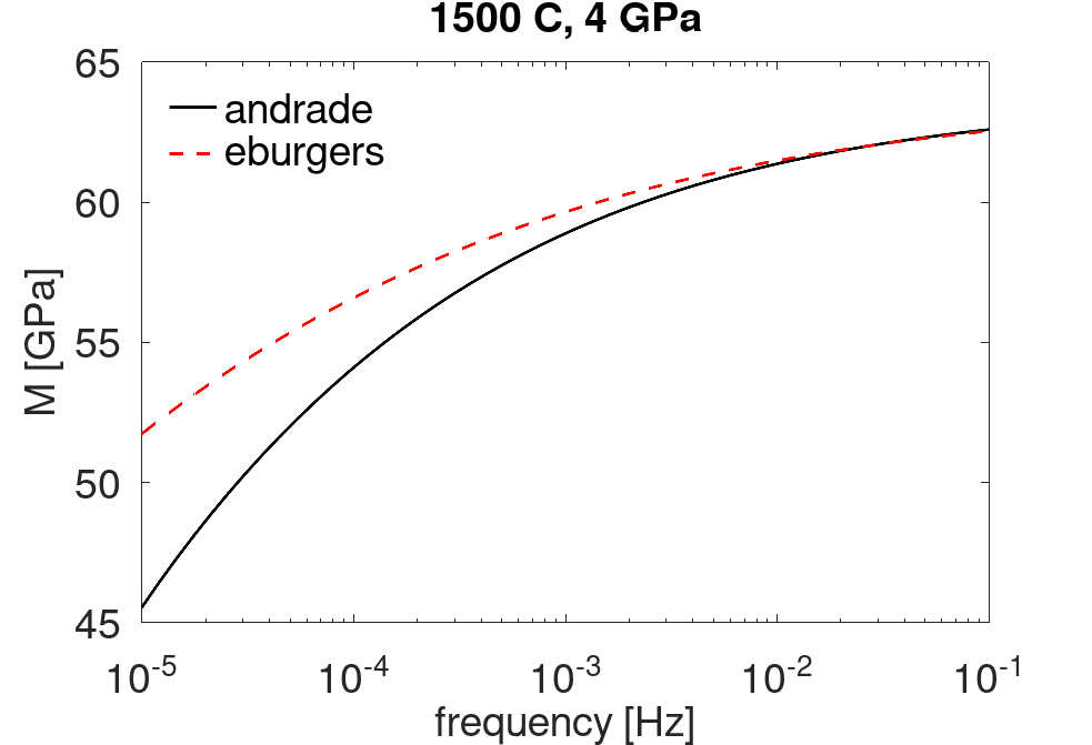
The remainder of the script pulls out some output variables to plot. For example, the following plots the effective relaxed shear modulus for the highest temperature and pressure of interest for our two methods:

figure('Position', [30 30 630 430]) % [x y width height]
iT = numel(T_K_1d);
iP = numel(P_GPa_1d);
f = VBR.in.SV.f;
semilogx(f, squeeze(VBR.out.anelastic.andrade_psp.M(iP, iT, :)/1e9), 'k','displayname', 'andrade', 'linewidth',1.5)
hold all
semilogx(f, squeeze(VBR.out.anelastic.eburgers_psp.M(iP, iT, :)/1e9),'--r', 'displayname', 'eburgers', 'linewidth',1.5)
legend('location', 'NorthWest', 'Box', 'off')
xlabel('frequency [Hz]')
ylabel('M [GPa]')
title('1500 C, 4 GPa')
set(findall(gcf,'-property','FontSize'),'FontSize',18)

png

Summary

With the new ability to directly specify the unrelaxed moduli used by the VBRc, it’s now a lot easier to couple your VBRc workflows with other tools out there that calculate unrelaxed moduli more accurately than the what is included in the VBRc. This also allows you to include more compositional variations in the VBRc (with the important caveat that the anelastic calculation assumes pure olivine…). The above example demonstrates this new feature entirely in MATLAB by using the Abers and Hacker (2016) MATLAB toolbox to calculate the unrelaxed moduli and density, which are then used as inputs to the VBRc.

References

Abers, G. A., and B. R. Hacker (2016), A MATLAB toolbox and Excel workbook for calculating the densities, seismic wave speeds, and major element composition of minerals and rocks at pressure and temperature, Geochem. Geophys. Geosyst., 17, 616–624, doi:10.1002/2015GC006171.
Hacker, B. R., and G. A. Abers (2004), Subduction Factory 3: An Excel worksheet and macro for calculating the densities, seismic wave speeds, and H2O contents of minerals and rocks at pressure and temperature, Geochem. Geophys. Geosyst., 5, Q01005, doi:10.1029/2003GC000614.
Isotta, E., Peng, W., Balodhi, A., and Zevalkink, A (2023), Elastic Moduli: a Tool for Understanding Chemical Bonding and Thermal Transport in Thermoelectric Materials, Angew. Chem. Int. Ed., 62, e202213649, doi:10.1002/anie.202213649.
Jackson, I., and Faul, U. (2010), Grainsize-sensitive viscoelastic relaxation in olivine: Towards a robust laboratory-based model for seismological application, Physics of the Earth and Planetary Interiors, 183, 1–2, doi:10.1016/j.pepi.2010.09.005.