Adding streamlines to a volume rendering in yt

I recently fielded a question on the yt slack about adding streamlines to a volume rendering in yt and decided it was worth documenting the solution a bit more!

RenderSource objects in yt’s volume rendering

Let’s start with an overview of the different representations of data in the volume rendering API in yt. The render_source module:

yt.visualization.volume_rendering.render_source`

has a number of objects for different data types based on a common RenderSource object that determines how the 3D rendering engine sample and composite data. The RenderSource types are divided into OpaqueSource and VolumeSource objects:

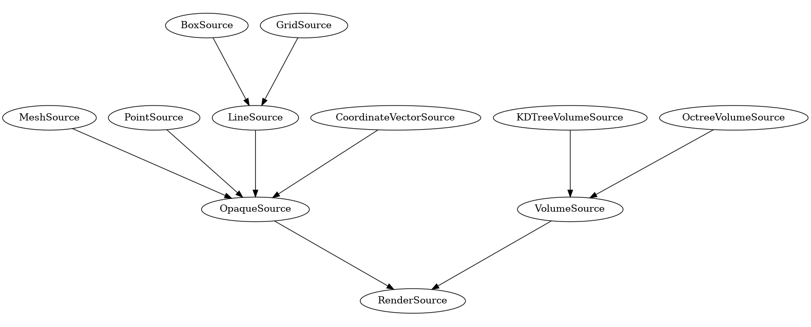
The VolumeSource objects (usually initialized via the create_volume_source function) are the volume rendering components while the OpaqueSource objects are additional annotations.

As a quick aside, the above graph was generated with the inheritance-explorer (link) package:

import inheritance_explorer as ie
from yt.visualization.volume_rendering.render_source import RenderSource
rs = ie.ClassGraphTree(RenderSource)
g = rs.graph(ratio=.4)
g.write_png('RenderSources.png')

Building curves with LineSource objects

So to add streamlines, we’ll want to use the LineSource in particular. This let’s you add lines, specified by start and end points to a volume rendering scene. The tricky part is that to we’ll need to split up our 3D curves into a series of line segments.

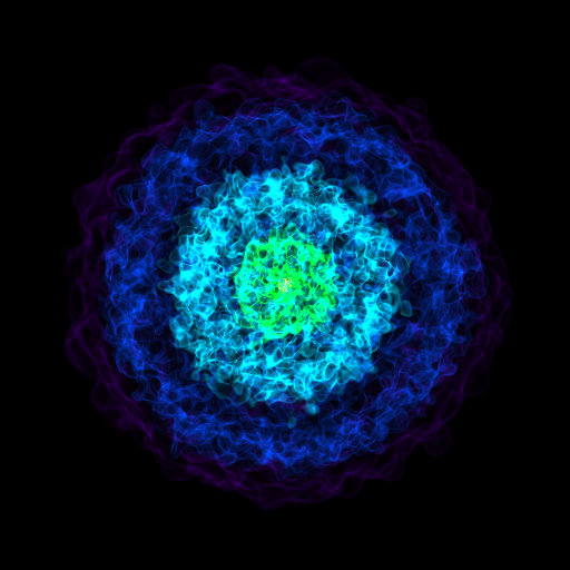
First, let’s build a base volume rendering

import yt
ds = yt.load("IsolatedGalaxy/galaxy0030/galaxy0030")
sc = yt.create_scene(ds)
sc.camera.zoom(3)
sc.show(sigma_clip=4)

So to use the LineSource, we need to provide a list of start and end points. The yt docs demonstrate this with random lines (link), but we can also create a continuous curve by stitching together multiple line segments:

import numpy as np
vertices = []
vert = ([0.5, 0.5, 0.5], [0.6, 0.52, 0.52])
vertices.append(vert)
vert_2 = (vert[-1], [0.3, 0.2, 0.48])
vertices.append(vert_2)
vertices = np.array(vertices)

Note that we’re simply setting the start of each consecutive line segment to the end of the prior segment:

print(vertices)
array([[[0.5 , 0.5 , 0.5 ],
        [0.6 , 0.52, 0.52]],

       [[0.6 , 0.52, 0.52],
        [0.3 , 0.2 , 0.48]]])

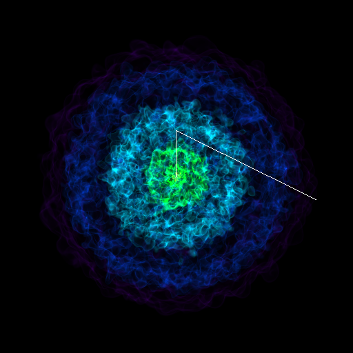
Let’s add this to our rendering:

colors = np.ones([vertices.shape[0], 4])    
colors[:, -1] = 0.1
ls = LineSource(vertices, colors)    
sc.add_source(ls)
sc.render()
sc.show(sigma_clip=4)

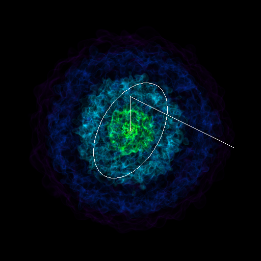
To add a continuous curve, we’ll take a our position array and split it into a series of line segments (I’m saying “continuous” here despite the fact that we’re still dealing with discrete positions… but if you sample at a high enough rate the curves will look smooth).

So, let’s create an arbitrary curve that we want to add. The following places a circle in the x-y plane centered in the z plane:

r = 0.1
theta = np.linspace(0, np.pi*2, 100)
x = r * np.cos(theta) + 0.5
y = r * np.sin(theta) + 0.5
z = np.full(x.shape, 0.5)
pos = np.column_stack([x, y, z])
print(pos[:3])

[[0.6        0.5        0.5       ]
 [0.59979867 0.50634239 0.5       ]
 [0.59919548 0.51265925 0.5       ]]

Now we’ll write a function to take that position array and split it up into a bunch of line segments.

def segment_a_curve(pos_i):
    index_range = np.arange(0, pos_i.shape[0])
    line_indices = np.column_stack([index_range, index_range]).ravel()[1:-1]

    line_segments = pos_i[line_indices, :]
    n_line_segments = int(line_segments.size/6)
    return line_segments.reshape((n_line_segments, 2, 3))
segmented = segment_a_curve(pos)

All that fancy indexing simply creates a series of vertices like we had in the simpler case, with the start points of each vertex being the end point of the prior:

print(segmented[:3])
[[[0.6        0.5        0.5       ]
  [0.59979867 0.50634239 0.5       ]]

 [[0.59979867 0.50634239 0.5       ]
  [0.59919548 0.51265925 0.5       ]]

 [[0.59919548 0.51265925 0.5       ]
  [0.59819287 0.51892512 0.5       ]]]

while not ideal in that we’re doubling the memory used for our curve, it does let us add our curves…

colors = np.ones([segmented.shape[0], 4])    
colors[:, -1] = 0.1
ls = LineSource(segmented, colors)    
sc.add_source(ls)
sc.render()
sc.show(sigma_clip=4)

Adding streamlines

Finally, we can get back to actually adding our streamlines. First, let’s calculate some streamline positions! The following function creates random starting points within a radial distance of 0.1 to 0.2 from the domain center:

def get_streamline_starting_pos(N):    
    c = ds.domain_center
    rng = np.random.default_rng()
    r = rng.uniform(low=0.1, high=0.2, size=(N,))
    theta = rng.uniform(low=0, high=2*np.pi, size=(N,))
    phi = rng.uniform(low=0, high=np.pi, size=(N,))

    z = r * np.cos(phi)
    xy = r * np.sin(phi)
    x = xy * np.cos(theta)
    y = xy * np.sin(theta)

    offset = np.column_stack([x, y, z])
    pos = c + ds.arr(offset, 'code_length')
    return pos

pos = get_streamline_starting_pos(10)

To build our streamlines, we’re going to first initialize an AMRKDTree – this is simply to save time since we can re-use it when we re-calculate streamlines later on and save some initialization time. You can skip this step if you don’t mind waiting for the KDTree to rebuild:

from yt.utilities.amr_kdtree.api import AMRKDTree

x_field = ("gas", "velocity_x")
y_field = ("gas", "velocity_y")
z_field = ("gas", "velocity_z")

volume = AMRKDTree(ds)
volume.set_fields(
    [x_field, y_field, z_field], [False, False, False], False
)
volume.join_parallel_trees()

Aaaand now let’s actually get those streamlines!!

streamlines = Streamlines(
    ds,
    pos,
    x_field, y_field, z_field,
    length=1.0 * Mpc,
    get_magnitude=True,
    volume=volume
)
streamlines.integrate_through_volume()

And create a new rendering… now we’ll iterate through each streamline and segment each one, create a line source and add it to the rendering:

sc = yt.create_scene(ds)
sc.camera.zoom(3)

for streamline in streamlines.streamlines:
    segmented_streamlines = segment_a_curve(streamline)
    colors = np.ones([segmented_streamlines.shape[0], 4])    
    colors[:, -1] = 0.01
    ls = LineSource(segmented_streamlines, colors)    
    sc.add_source(ls)

sc.render()
sc.show(sigma_clip=4)

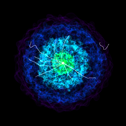
Woo! there it is.

When adding OpaqueSource objects, that alpha value can have a strong influence on the final image. Up above, this is set to 0.01 – if it’s higher then the lines will tend to swamp out the volume rendering and you’ll only see the streamlines. This takes a bit of trial and error to get right.

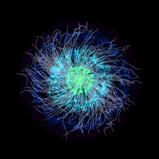
And just for fun, let’s try adding a bunch of streamlines. First, get our new starting positions:

pos = get_streamline_starting_pos(500)

and now a new Streamlines object (using the same volume as before):

streamlines = Streamlines(
    ds,
    pos,
    x_field, y_field, z_field,
    length=1.0 * Mpc,
    get_magnitude=True,
    volume=volume
)

and the integration (this step will take a while):

streamlines.integrate_through_volume()

Now, let’s rebuild our rendering again

sc = yt.create_scene(ds)
sc.camera.zoom(3)

for streamline in streamlines.streamlines:
    segmented_streamlines = segment_a_curve(streamline)
    colors = np.ones([segmented_streamlines.shape[0], 4])    
    colors[:, -1] = 0.01
    ls = LineSource(segmented_streamlines, colors)    
    sc.add_source(ls)

sc.render()
sc.show(sigma_clip=4)

yt_idv ?

As a final note, this is very similar to how I implemented the streamline functionality in yt_idv! The index manipulation is pretty much identical and then the vertex positions are passed down to the GPU where OpenGL draws the lines.

notebook

For convenience, I dropped all the above code into a notebook, available here.