A quick primer on volume rendering of geophysics data with yt
Over the past couple years I’ve worked on volume rendering of 3D geoscience data using yt in a number of ways. This post serves as quick primer on that work, with suggestions for how to get started and aspects that may be tricky!
Volume rendering?
When working with 3D volumetric data, scientists usually rely on visualizations that reduce the dimensionality of the data. This reduction could simply be a sampling like a 2D slice through a 3D volume or it could involve some operation like an integration that collapses one of the dimensions. It makes sense that we rely on lower dimensionality plots – ultimately we’re limited by our 2d media and until everyone has immersive 3D virtual environments we have to find a way to put our 3D data onto a 2D plane whether it’s paper or screen. But what if we could easily create renderings on a 2d page that inherently capture the 3d spatial relationships we’re interested in? Enter volume rendering!
Put very simply, volume rendering is a way of sampling a 3D volume by projecting parallel rays through the volume and aggregating data along each ray. But if we aggregate the data in the right way, we can actually retain information on spatial relationships! This way of projecting rays is derived from ray tracing in computer graphics and as such, a lot of the terminology and concepts tend to have computer graphiscy names (which will be unfamiliar to most physical scientists). For a very nice overview that doesn’t get too technical, check out Callahan et. al, 2008.
So of the two parts of volume rendering, ray projection and aggregation along rays, it is typically the aggregation that we have to think the most about. Since we’re not talking about optical ray tracing (where the rays are actual light rays that may bend and bounce), we don’t generally have to worry too much about the details of how the ray tracing works. The aggregation, however, is what controls our final image, and it is controlled by a transfer function. Let’s take a look at a rendering to explain it! The following is an example of a 3D volume rendering from Havlin et al. 2020 using the yt package:
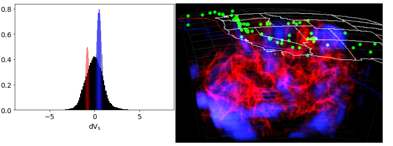
The right panel is our rendering and the left panel is the transfer function. The transfer function has two adjustable parameters: a transmission coefficient, alpha, and a color mapping. Here, we can see 2 gaussians (red and blue) centered at a narrow range of positive and negative velocity anomalies. At each step along each ray, the data is sampled, and then the transfer function is used to look up the color value and transmission coefficient for that data sample and then the color is blended with the cumulative value along the ray based on the transmission coefficient. The resulting image clearly preserves spatial relationships (the red fields are exterior to the blues) and we have a record of how the image was made (the transfer function).
In yt, you have direct control over the transfer function used. This is both awesome and challenging. It means that you will be able to check the sensitivity of your images to different transfer functions (awesome) and share your tailor-made transfer functions with others via code snippets (awesome) but it also means you have to figure out what to use for a transfer function (challenging).
Getting started
In this primer, I mostly present my general workflow to help you get started. While there are some code snippets, they are meant more to describe the process in general. For more fully worked examples you can check out the links below:
- Havlin et. al, EarthCube 2020 (summary, repository link, static notebook rendering): a self-contained notebook from the EarthCube 2020 annual meeting demonstrating volume rendering of a seismic tomography model of the upper mantle in the western U.S.
- Havlin et. al, AGU 2020 (repo link): an AGU “poster” full of notebooks demonstrating how to use yt with a range of geoscience data .
Additionally, I’ll refer to a number of repositories:
- yt: https://yt-project.org/ Even if you’re unfamiliar with astro datasets, it’s worth first working through the quick start and then reading the overview on volume rendering
- ytgeotools: a newish repositority still in early development to help facilitate using yt with geoscience data.
- yt_idv: yt’s latest interactive data exploration tool
Finally, you may prefer the initial draft of this post with less narrative that is available here.
general workflow for seismic data
So the easiest data to work with initially are IRIS EMC earth models. The main reason for this is that to use yt for volume rendering, the simplest approach is to use an already-gridded product. The following code snippets are intentionally incomplete: they are designed more to offer an overview of how to get started. For more complete examples, check out the links above.
To get started working with 3d data is to read the model data from native storage (e.g., a netcdf file) into yt. At present, the easiest way to do this is with in-memory dataset created using yt.load_uniform_grid() (docs link).
How to do that exactly depends (1) on your data and (2) what you’re going to do with the data. The second point relates to a current but important limitation of yt: volume rendering requires cartesian coordinates!
Loading the raw data
So even though volume rendering requires cartesian coordinates, it’s worth mentioning that you can load in your raw netcdf data in typical latitude, longitude and radius coordinates with yt. This is nice for making maps! To do this, we load the data as an internal_geographic dataset:
ds = yt.load_uniform_grid(data,
                          sizes,
                          1.0,
                          geometry=("internal_geographic", dims),
                          bbox=bbox)
where:
data: dictionary of field data arrays read from your netcdf
sizes: the shape of the field data
bbox: the bounding box
dims: the ordering of dimensions in the data arrays
Since we can’t volume render with this type of dataset, I won’t go over this much, but you can see this notebook for a full example or see this notebook for an fun example using obspy and yt together to sample along seismic raypaths.
At present, the main caveats of this method are:
- can only create fixed-depth maps (no cross-sections)
- still a little buggy (global models seem to work better than non-global models)
- no volume rendering
geo-volume rendering with yt
Now we get to it! Ok, so the first condition, mentioned above is that data must be in cartesian coordinates. So to do that, we have to interpolate the seismic model from geographic coordinates to a (uniform) cartesian grid.
Overall, my approach (in pseudo-python-code) is as follows:
1. convert the model’s lat, lon, depth arrays to geocentric cartesian coordinates:
lat, lon, radius = read_from_raw_data()
x, y, z = to_cartesian(lat, lon, radius)
once we have the raw grid points in cartesian, we
2. find the bounding box in cartesian coordinates:
cart_bbox = [
             [x.min(), x.max()],
             [y.min(), y.max()],
             [z.min(), z.max()],
            ]
If your latitude-longitude-radius ranges are small enough, you might be OK with stopping here and just treating your initial grid as uniform in cartesian. But in most cases if you do that you’ll get some unrealistic stretching (and it won’t work at all for global models), so we need to move on to interpolating.
3. Create a uniform grid to cover bounding box:
x_i = np.linspace(min_x, max_x, n_x)
y_i = np.linspace(min_y, max_y, n_y)
z_i = np.linspace(min_z, max_z, n_z)
4. find the data values at all those points
data_on_cart_grid = new array
for xv, yv, zv in np.meshgrid(x_i, y_i, z_i):
    data_on_cart_grid[xvi, yvi, zvi] = sample_the_data(xv, yv, zv)
This step is the most critical. Its the step that is most prone to computational limitations (the above loop is actually not a great idea, it will be very slow for reasonable n_x, n_y and n_z).
How to sample_the_data ?
So the approach I’ve taken is to use a KDtree for resampling. The first step here is to create a KDtree with the original cartesian coordinates:
tree = KDtree(x, y, z)
Then, for every point on the new cartesian grid, I use the KDtree to find the N closest points within some max distance, which are then averaged using inverse-distance weighting (IDW). This is nice because it’s pretty fast, but all of the extra tuneable parameters can be tricky to deal with and may introduce re-sampling errors. Depending on the resolution of the covering grid relative to the underlying data and how many missing values the underlying data contains, there can often be clear artifacts or just missing data entirely. So this is definitely a step to experiment with further as you start to generate images.
Once data is sampled
Once the data is interpolated to the new uniform cartesian grid, we can use yt.load_uniform_grid:
data = {"dvs": dvs_on_cartesian}
bbox = cart_bbox
sizes = dvs_on_cartesian.shape
ds = yt.load_uniform_grid(data, sizes, 1.0)
And now use volume rendering!
The above workflow is the basis for my work presented at AGU2020 and EarthCube2020, both of which rely on an initial helper package called yt_velmodel_vis. While that package should still work, I’ve moved development over to a new package called ytgeotools.
geo-volume rendering in practice:
The examples here rely on the new ytgeotools package which helps to streamline the above process of initially loading data into yt while adding some additional analysis functionality. The basic usage for loading an IRIS netcdf file into a yt dataset is:
import yt
from ytgeotools.seismology.datasets import XarrayGeoSpherical
filename = "IRIS/GYPSUM_percent.nc"

# to get a yt dataset for maps:
ds_yt = XarrayGeoSpherical(filename).load_uniform_grid()

# to get a yt dataset on interpolated cartesian grid:
ds = XarrayGeoSpherical(filename)
ds_yt_i = ds.interpolate_to_uniform_cartesian(
    ["dvs"],
    N=50,
    max_dist=50,
    return_yt=True,
)
should be useable for any IRIS EMC netcdf file to get a yt dataset.
The work is still in an early stage and installation is not yet streamlined, so you need to install two packages from source in the following order:
To use any of the mapping functionality, you also need cartopy so you may want to use a conda environment to facilitate that installation.
So to get started with ytgeotools, first download or clone the two packages above, make sure conda environment is active, then cd into yt_idv and install from source with
$ python pip install .
Repeat that for ytgeotools.
Test installation: from a python shell, try:
>>> import yt_idv
>>> import ytgeotools
>>> import yt
There may be some more missing dependencies to install… hopefully this will be further streamlined soon!
manual volume rendering
The AGU and EarthCube notebooks use the standard yt volume rendering interfaces. Excerpted from those notebooks, the typical workflow to create an image using ytgeotools would look like:
import yt
from ytgeotools.seismology.datasets import XarrayGeoSpherical

# load the cartesian dataset
ds_raw = XarrayGeoSpherical(filename)
ds = ds_raw.interpolate_to_uniform_cartesian(
    ["dvs"],
    N=50,
    max_dist=50,
    return_yt=True,
)

# create the scene (loads full dataset into the scene for rendering)
sc = yt.create_scene(ds, "dvs")

# adjust camera position and orientation (so "up" is surface)
x_c=np.mean(bbox[0])
y_c=np.mean(bbox[1])
z_c=np.mean(bbox[2])
center_vec = np.array([x_c,y_c,z_c])
center_vec = center_vec / np.linalg.norm(center_vec)
pos=sc.camera.position
sc.camera.set_position(pos,north_vector=center_vec)

# adjust camera zoom
zoom_factor=0.7 # < 1 zooms in
init_width=sc.camera.width
sc.camera.width = (init_width * zoom_factor)

# set transfer function
# initialize the tf object by setting the data bounds to consider
dvs_min=-8
dvs_max=8
tf = yt.ColorTransferFunction((dvs_min,dvs_max))

# set gaussians to add
TF_gaussians=[
    {'center':-.8,'width':.1,'RGBa':(1.,0.,0.,.5)},
    {'center':.5,'width':.2,'RGBa':(0.1,0.1,1.,.8)}
]

for gau in TF_gaussians:
    tf.add_gaussian(gau['center'],gau['width'],gau['RGBa'])

source = sc.sources['source_00']
source.set_transfer_function(tf)

# adjust resolution of rendering
res = sc.camera.get_resolution()
res_factor = 2
new_res = (int(res[0]*res_factor),int(res[1]*res_factor))
sc.camera.set_resolution(new_res)

# if in a notebook
sc.show()

# if in a script
sc.save()
As mentioned above, there can be a lot of trial and error for transfer functions and also camera positioning. And making videos requires adjusting the camera position, saving off the images and then stitching together the frames with a different tool.
interactive volume rendering
ytgeotools is built to easily interface with yt’s latest interactive rendering environment, yt_idv. It’s great for getting a sense of whether or not the interpolation is working. At present, the transfer function behavior is slightly different: the custom transfer function functionality is not fully working yet, but the maximum value and projection functions work! The following script loads a dataset and spawns a rendering environment:
import numpy as np
import yt_idv
from ytgeotools.seismology.datasets import XarrayGeoSpherical


def refill(vals):
    # vals will be a numpy array containing the data on the
    # the interpolated grid. We can modify/mask it any way
    # we want here and return it.
    vals[np.isnan(vals)] = 0.0
    vals[vals > 0] = 0.0
    return vals


filename = "IRIS/NWUS11-S_percent.nc"
ds = XarrayGeoSpherical(filename)
ds_yt = ds.interpolate_to_uniform_cartesian(
    ["dvs"],
    N=50,
    max_dist=50,
    return_yt=True,
    rescale_coords=True, ## IMPORTANT to rescale!
    apply_functions=[refill, np.abs],
)

rc = yt_idv.render_context(height=800, width=800, gui=True)
sg = rc.add_scene(ds_yt, "dvs", no_ghost=True)
rc.run()
For initially loading in seismic data that are velocity anomalies, I often find it helpful to mask out positive and negative anomalies and investigate them separately. So in the interpolate_to_uniform_cartesian method above I included the option to pass in function handles. These functions will get run after the re-gridding and must accept and return a single numpy array.
annotations:
Finally, it’s important to be able to add georeferenced annotations to the renderings in order to orient oneself. When using yt’s manual plotting interface we can do that with Point and Line sources:
from yt.visualization.volume_rendering.api import LineSource, PointSource
The EarthCube/AGU notebooks have some helper functions to streamline this, so check those out for examples. One important note is that adding the Point and Line sources can affect the overall brightness of the scene, which demands some trial and error to adjust the opacity of the sources so that they do not wash out the volume rendering.
Recent work in yt_idv added the ability to add arbitrary curves, so ytgeotools will soon have some extra functionality to make it easier to add georeferenced data to the interactive plots as well.
summary
This post was meant as gentle introduction to volume rendering in yt. I hope you found it useful! If you’re interested in helping to develop ytgeotools, contributions via github pull request are welcome!