loading 2D datasets in yt
yt has a number of ways to load in generic array data as yt datasets and occasionally I’ve found myself wanting to load in 2D arrays for various reasons. Turns out it’s very easy to do, but the docs don’t explicitly cover the use case. So here’s a quick how-to!
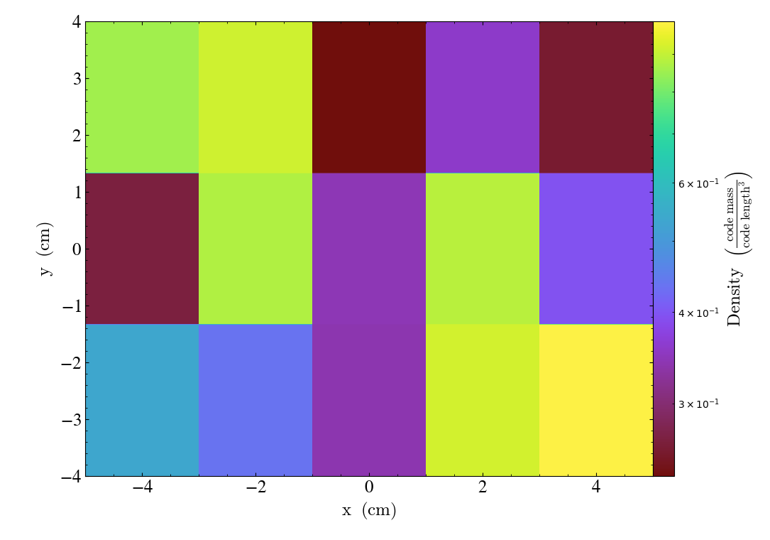
loading 2D data with load_uniform_grid
So even 2D datasets in yt are 3D under the hood – this means that to load 2D data we need to provide some dummy values for the 3rd dimension. And when slicing, you’ll want to slice normal to the unused dimensions (z in this case).
import yt
import numpy as np

shp = (5, 3, 1)
data = {"density": np.random.random(shp)}
ds = yt.load_uniform_grid(data, shp, geometry=("cartesian", ("x", "y", "z")))
yt.SlicePlot(ds, "z", ("stream", "density"))
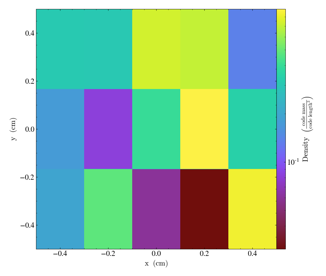
When providing a bbox or geometry, you also need to add account for the dummy dimension. The following loads the first dimension as the dummy dimension, but then uses the geometry argument to again set z to be the dummy dimension:
shp = (1, 5, 3)
bbox = np.array([[-0.5, 0.5], [-4., 4.], [-5., 5.], ])
data = {"density": np.random.random(shp)}
ds = yt.load_uniform_grid(data,
                          shp,
                          geometry=("cartesian", ("z", "y", "x")),
                          bbox=bbox)
yt.SlicePlot(ds, "z", ("stream", "density"))
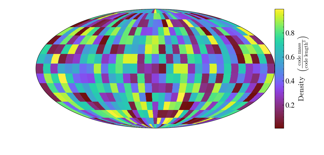
This also works just fine with other geometries:
# requires cartopy
shp = (15, 33, 1)
data = {"density": np.random.random(shp)}
ds = yt.load_uniform_grid(data,
                          shp,
                          bbox=np.array([[-90, 90], [-180, 180], [-.5, 0.5]]),
                          geometry=("geographic",
                                    ("latitude", "longitude", "altitude"))
                         )
slc = yt.SlicePlot(ds, "altitude", ("stream", "density"))
slc.set_log(("stream", "density"), False)
slc.show()
loading 2D AMR data with load_amr_grids
It’s also possible to use the same approach for loading in 2D AMR data: when adding grid definitions, just keep one of the dimensions fixed. Following the example from the yt docs:
import numpy  as np
import yt

grid_data = [
    dict(
        left_edge=[0.0, 0.0, 0.],
        right_edge=[1.0, 1.0, 1.],
        level=0,
        dimensions=[32, 32, 1],
    ),
    dict(
        left_edge=[0.25, 0.25, 0.],
        right_edge=[0.75, 0.75, 1.],
        level=1,
        dimensions=[32, 32, 1],
    ),
]


for g in grid_data:
    g["density"] = (np.random.random(g["dimensions"]) * 2 ** g["level"], "g/cm**3")


bbox = np.array([[0., 1.], [0., 1.], [0., 1.]])

ds = yt.load_amr_grids(grid_data, [32, 32, 1], bbox=bbox)
slc = yt.SlicePlot(ds, "z", ("gas", "density"))
slc.show()
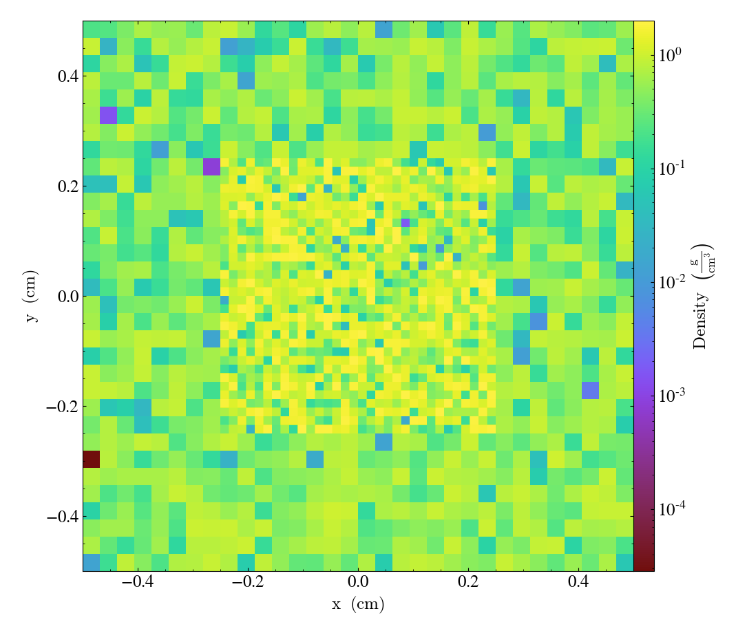
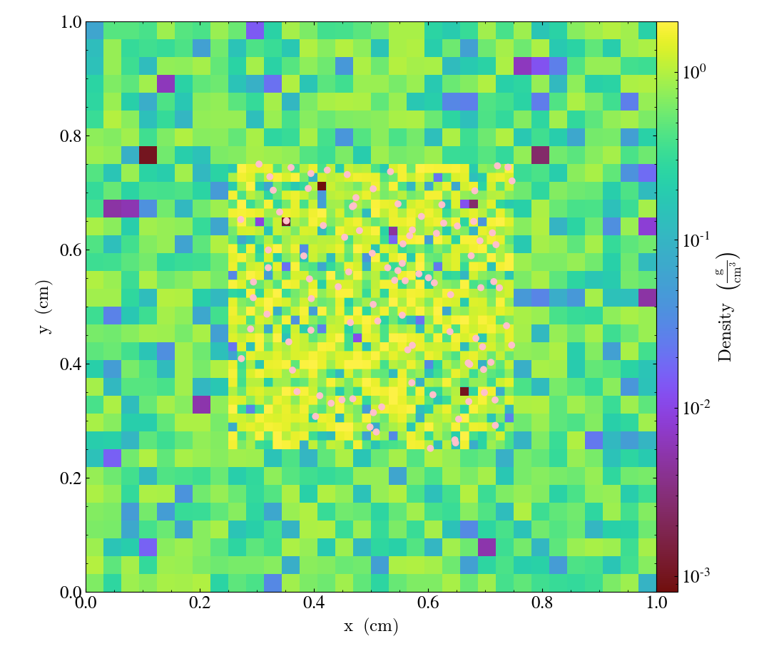
adding particles
It’s also worth noting that when adding particles, you should add them at the midpoint of the dummy dimensions. In the previous example, that would mean adding them at z=0.5 (or the mean of the bbox in the z dimension)
grid_data = [
    dict(
        left_edge=[0.0, 0.0, 0.],
        right_edge=[1.0, 1.0, 1.],
        level=0,
        dimensions=[32, 32, 1],
    ),
    dict(
        left_edge=[0.25, 0.25, 0.],
        right_edge=[0.75, 0.75, 1.],
        level=1,
        dimensions=[32, 32, 1],
    ),
]

for g in grid_data:
    g["density"] = (np.random.random(g["dimensions"]) * 2 ** g["level"], "g/cm**3")


# only adding particles at the highest level, set empty here
grid_data[0]["particle_position_x"] = (np.array([]),"code_length")
grid_data[0]["particle_position_y"] = (np.array([]), "code_length")
grid_data[0]["particle_position_z"] = (np.array([]), "code_length")

nparticles=100
grid_data[1]["particle_position_x"] = (
    np.random.uniform(low=0.25, high=0.75, size=nparticles),
    "code_length",
)
grid_data[1]["particle_position_y"] = (
    np.random.uniform(low=0.25, high=0.75, size=nparticles),
    "code_length",
)
# set z position to mean of z dimension of the bbox!
grid_data[1]["particle_position_z"] = (
    np.full((nparticles,), np.mean(bbox[2,:])),
    "code_length",
)

bbox = np.array([[0., 1.], [0., 1.], [0., 1.]])

ds = yt.load_amr_grids(grid_data, [32, 32, 1], bbox=bbox)
slc = yt.SlicePlot(ds, "z", ("gas", "density"), origin='native')
slc.annotate_particles(1, p_size=50.0, col="Pink")
slc.show()