Overview of yt_xarray#
yt_xarray is a package built to facilitate data transfer between xarray and yt. Its primary implementation is through an xarray accessor object, accessible off of any
xarray dataset object. Given an xarray dataset, ds, the primary method ds.yt.load_grid
will load a field or subset of fields from the xarray dataset within a wrapping yt dataset:
import yt_xarray

# load a standard xarray dataset
ds = yt_xarray.open_dataset("path/to/your/dataset.nc") # or xarray.open_dataset
# initialize a yt dataset wrapper
yt_ds = ds.yt.load_grid(fields=(['list','of','fields']))
yt_xarray is designed to minimize and delay copying of data where possible. As such, references to the original xarray dataset are maintained within the wrapping yt dataset and data is only read on-demand. For gridded datasets, yt processes grids independently, resulting in a delayed, on-demand read of index ranges in the underlying xarray dataset. When that xarray dataset is chunked with Dask or Zarr, the chunks will be contained within yt grids and only read on demand.
Recent Improvements#
A number of recent updates to both yt_xarray and yt have simplified using yt with xarray datasets.
First, a number of functions from the yt API have been exposed from within the yt_xarray .yt
accessor object, including: SlicePlot, ProjectionPlot, PhasePlot and ProfilePlot, allowing the user to skip the intermediate step of creating a yt dataset object.
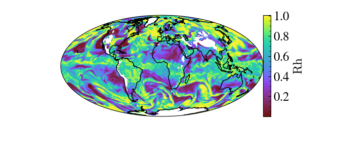
The following example creates a slice plot of a MERRA-2 reanalysis file (Global Modeling and Assimilation Office, 2015):
import yt_xarray
import cartopy.feature as cfeature
import numpy as np

dsx = yt_xarray.open_dataset("sample_nc/MERRA2_100.inst3_3d_asm_Np.19800120.nc4")
dsx0 = dsx.isel({'time':0})
slc = dsx0.yt.SlicePlot('altitude', 'RH', center=(800, 0.,0.))
slc.set_log('RH', False)
slc.render()
slc.plots['RH'].axes.add_feature(cfeature.COASTLINE)
slc.show()
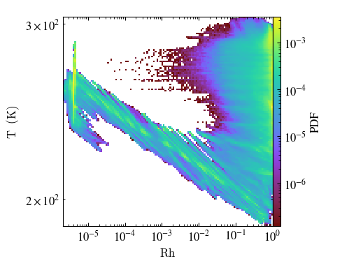
The following code creates a yt.PhasePlot, a 2D binned statistic plot by binning the temperature (T) and relative humidity (RH) variables across the whole dataset. The 3rd variable is the binned field (in this case an array of ones) and values are summed within bins (by setting weight_field=None) and normalized by their totals (fractional=True), resulting in a global 2D probability distribution of T vs RH.
# add a field fo
ones_da = xr.DataArray(np.ones(dsx0.RH.shape), dims=dsx0.RH.dims)
dsx0['ones_field'] = ones_da

pp = dsx0.yt.PhasePlot('RH', 'T', 'ones_field', weight_field=None, fractional=True, figure_size=(3,3))
pp.set_colorbar_label('ones_field','PDF')
pp.set_font_size(12)
pp.show()
pp.save('slice_images/merra2_phase_plot.png')
Within yt, there have also been improvements to plot annotations for geopgraphic data (released in yt v4.4.0) and in-progress arbitrary cutting planes which will allow cross-section construction (yt PR#4847)